Chapter 10 Other resources
In this chapter, we provide a curated list of additional resources that complement the TCMDATA package for TCM network pharmacology research. These include databases, tools, and R packages that can be integrated into your analysis workflow for enhanced data retrieval, processing, and visualization.
10.1 Additional databases
10.1.1 TF–gene interactions (DoRothEA)
Transcription factors (TFs) are master regulators that control gene expression by binding to specific DNA sequences. In network pharmacology, understanding TF–target relationships is crucial for identifying upstream regulators of disease-associated genes and constructing comprehensive regulatory networks.
TCMDATA provides a curated dataset of high-confidence TF–target interactions derived from the DoRothEA database[1]. The dataset includes interactions at confidence levels A, B, and C for both Human and Mouse:
| Confidence | Evidence Source | Description |
|---|---|---|
| A | Literature-curated | High confidence; manually curated from publications |
| B | ChIP-seq evidence | Moderate confidence; supported by chromatin immunoprecipitation data |
| C | TFBS + ChIP-seq | Medium confidence; predicted binding sites validated by ChIP-seq |
User can access this data via data("tf_targets"):
#> # A tibble: 10 × 5
#>    Species TF    Target   Confidence Mode_of_Regulation
#>    <chr>   <chr> <chr>    <chr>                   <dbl>
#>  1 Human   AHR   CYP1A1   C                           1
#>  2 Human   AHR   CYP1A2   C                           1
#>  3 Human   AHR   CYP1B1   C                           1
#>  4 Human   AHR   FOS      C                           1
#>  5 Human   AHR   MYC      C                           1
#>  6 Human   AHR   UGT1A6   C                           1
#>  7 Human   AHR   ASAP1    C                           1
#>  8 Human   AHR   ERG      C                           1
#>  9 Human   AHR   VGLL4    C                           1
#> 10 Human   AHR   ARHGAP15 C                           1
The Mode_of_Regulation column indicates whether the TF activates (1) or inhibits (-1) the target gene, enabling construction of signed regulatory networks.
10.1.1.1 Application example
This dataset is particularly useful for:
- TF enrichment analysis — Identify which TFs are significantly associated with your disease targets.
- Regulatory network construction — Build TF → target → disease networks to reveal upstream regulatory mechanisms.
- Integration with TCM networks — Link TCM targets to their upstream TFs, extending the herb → molecule → target → TF cascade.
10.1.2 Gut microbiota–host interactions (GutMGene)
The gut microbiome plays a critical role in human health by producing metabolites that modulate host physiology. These microbial metabolites, which are similar to TCM active compounds, are small molecules that interact with host target proteins. This “Gut Microbiota → Metabolite → Host Target” axis provides a natural extension to the classical TCM network pharmacology paradigm, enabling researchers to explore how gut microbiota may mediate or modulate the therapeutic effects of herbal medicines.
TCMDATA integrates comprehensive gut microbiota–metabolite–target interaction data from the GutMGene v2.0 database[2]. The dataset covers both Human and Mouse and includes:
- Bacteria–Metabolite relationships: Which gut bacteria produce specific metabolites
- Metabolite–Target relationships: Which host genes are regulated by microbial metabolites
- Interaction type: Whether the metabolite activates or inhibits the target
#>                  Bacteria Bacteria_ID Metabolite Metabolite_ID Target Target_ID
#> 1  Christensenella minuta      626937    Acetate           175  FFAR3      2865
#> 2  Christensenella minuta      626937    Acetate           175  FFAR2      2867
#> 3  Christensenella minuta      626937    Acetate           175   CCL2      6347
#> 4  Christensenella minuta      626937    Acetate           175   LGR5      8549
#> 5  Christensenella minuta      626937    Acetate           175   ALPI       248
#> 6  Christensenella minuta      626937    Acetate           175   MUC2      4583
#> 7  Christensenella minuta      626937    Acetate           175  DCLK1      9201
#> 8  Christensenella minuta      626937    Acetate           175   OCLN 100506658
#> 9  Christensenella minuta      626937    Acetate           175  CLDN3      1365
#> 10 Christensenella minuta      626937    Acetate           175   TJP1      7082
#>    Interaction PMID_Bac_Met PMID_Met_Target
#> 1   activation     21357455        28322790
#> 2   activation     21357455        28322790
#> 3   inhibition     21357455        28322790
#> 4   activation     21357455        32240190
#> 5   activation     21357455        32240190
#> 6   activation     21357455        32240190
#> 7   activation     21357455        32240190
#> 8   activation     21357455        32240190
#> 9   activation     21357455        32240190
#> 10  activation     21357455        32240190
data("gutMGene") loads a list with two data frames: gut_axis_human and gut_axis_mouse.
10.1.2.1 Application example: Gut–TCM integration
Since microbial metabolites and TCM active compounds are both small molecules targeting host proteins, you can integrate GutMGene with TCM network analysis to explore:
- Shared targets — Do TCM compounds and gut metabolites regulate the same host genes?
- Synergistic effects — Can TCM herbs modulate gut microbiota composition, thereby influencing metabolite production?
- Multi-layer networks — Construct Bacteria → Metabolite → Target → Pathway networks analogous to Herb → Molecule → Target → Pathway networks.
10.1.2.2 Network visualization with ggtangle
The tripartite structure of gut microbiota data (Bacteria → Metabolite → Target) mirrors the TCM network paradigm (Herb → Molecule → Target). Below we demonstrate how to visualize this relationship using ggtangle:
library(TCMDATA)
library(dplyr)
library(igraph)
library(ggtangle)
library(ggplot2)
library(ggrepel)

data("gutMGene")

# Select one bacterium with multiple metabolites and targets
bac_name <- "Bifidobacterium longum"

gut_sub <- gutMGene$gut_axis_human |>
  filter(Bacteria == bac_name, !is.na(Metabolite), !is.na(Target))

# Sample targets to keep the network readable
set.seed(2026)
gut_sub <- gut_sub |>
  group_by(Metabolite) |>
  slice_sample(n = 8) |>
  ungroup()

# Build edges: Bacteria → Metabolite → Target
edges <- bind_rows(
  gut_sub |> distinct(from = Bacteria, to = Metabolite),
  gut_sub |> distinct(from = Metabolite, to = Target)
)

# Node attributes
nodes <- tibble(name = unique(c(edges$from, edges$to))) |>
  mutate(type = case_when(
    name == bac_name ~ "Bacteria",
    name %in% gut_sub$Metabolite ~ "Metabolite",
    TRUE ~ "Target"
  ))

# Build and plot network
g <- graph_from_data_frame(edges, directed = FALSE, vertices = nodes)

set.seed(2026)
ggplot(g, layout = "fr") +
  geom_edge(alpha = 0.15, color = "grey55") +
  geom_point(aes(color = type, shape = type, size = type), alpha = 0.9) +
  geom_text_repel(
    aes(label = name),
    size = 3, max.overlaps = 30, segment.alpha = 0.3
  ) +
  scale_color_manual(
    values = c("Bacteria" = "#E64B35", "Metabolite" = "#4DBBD5", "Target" = "#00A087"),
    name = "Node Type"
  ) +
  scale_shape_manual(
    values = c("Bacteria" = 18, "Metabolite" = 15, "Target" = 16),
    name = "Node Type"
  ) +
  scale_size_manual(
    values = c("Bacteria" = 6, "Metabolite" = 5, "Target" = 3.5),
    name = "Node Type"
  ) +
  theme_void() +
  theme(
    legend.position = "right",
    legend.title = element_text(face = "bold", size = 11),
    legend.text = element_text(size = 10)
  )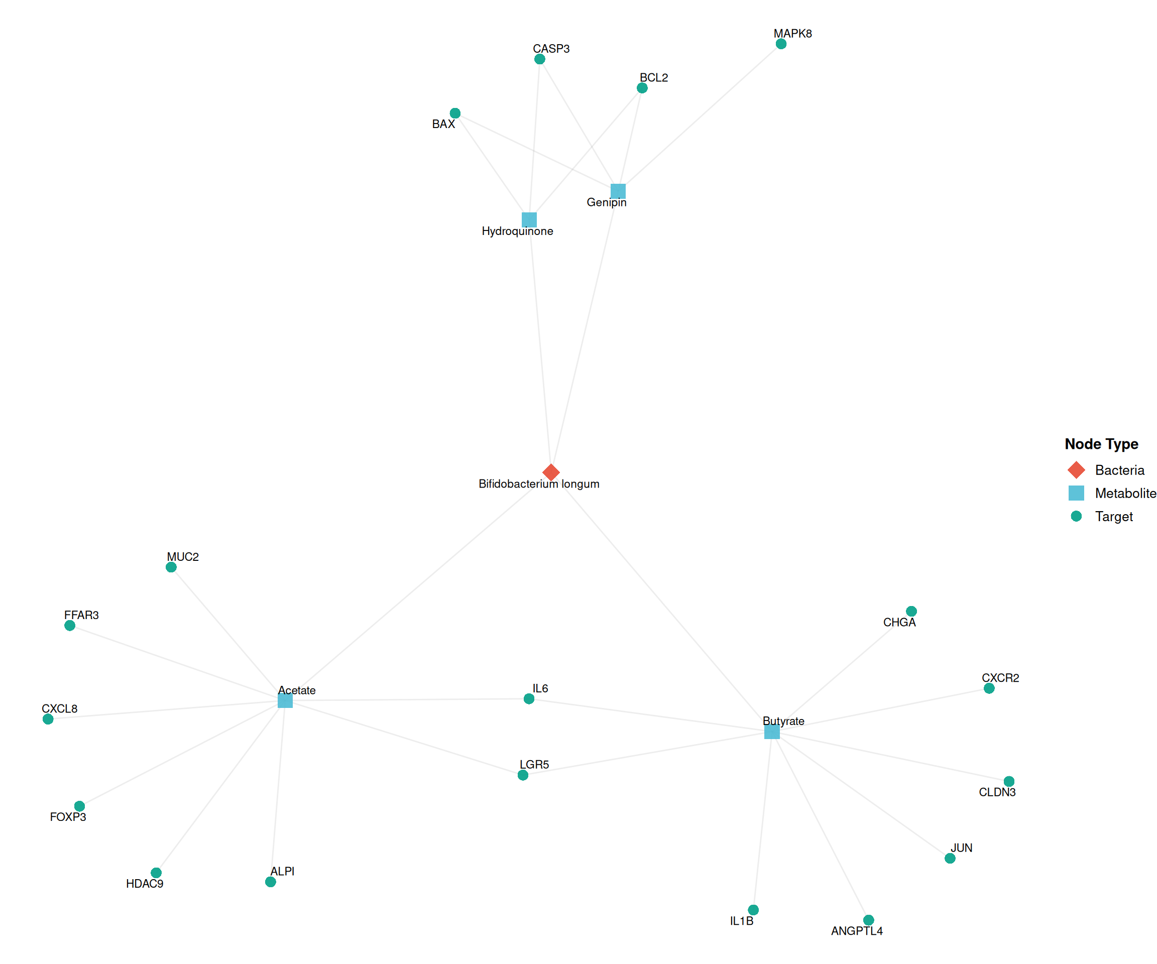
The network reveals the multi-target nature of gut microbial metabolites—analogous to TCM active compounds—where a single metabolite (e.g., Acetate, Butyrate) can modulate multiple host genes through distinct signaling pathways.
10.2 Additional visualization
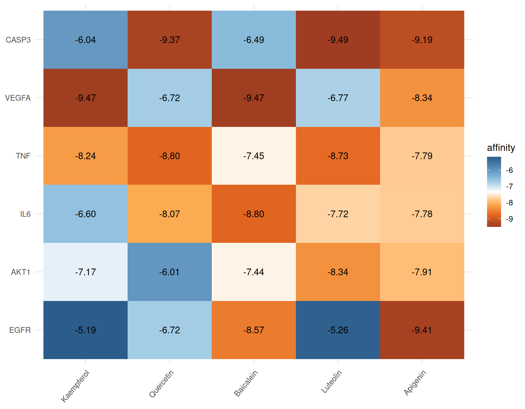
10.2.1 Heatmap for molecular docking results
Molecular docking is a key computational method in network pharmacology for validating interactions between TCM active compounds and target proteins. After performing docking simulations (e.g., with AutoDock Vina), users typically obtain a matrix of binding affinities (kcal/mol) where more negative values indicate stronger binding.
TCMDATA provides ggdock() for visualizing docking results as heatmaps. The function supports both dot plots and tile plots, with flexible color palettes and optional affinity labels.
library(TCMDATA)

# Generate demo docking data
set.seed(2026)
molecules <- c("Quercetin", "Kaempferol", "Luteolin", "Apigenin", "Baicalein")
targets <- c("AKT1", "EGFR", "TNF", "IL6", "VEGFA", "CASP3")

dock_matrix <- matrix(
  runif(length(molecules) * length(targets), min = -9.5, max = -4.5),
  nrow = length(targets),
  dimnames = list(targets, molecules)
)

# Dot plot
ggdock(dock_matrix, order = "median", type = "dot", point_size = 10)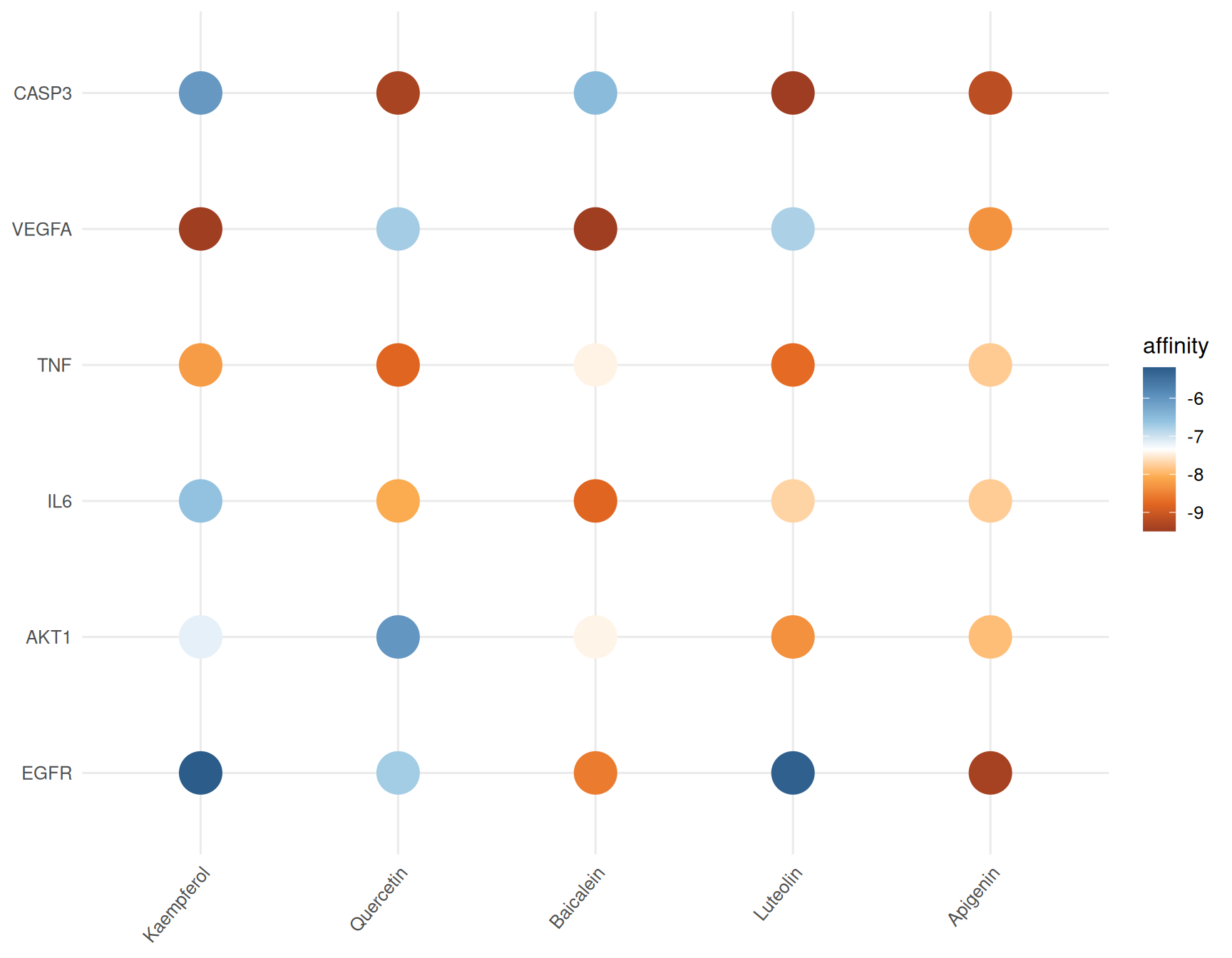
Also, you can try tile plot with affinity labels:
10.3 References
Garcia-Alonso L, Holland CH, Ibrahim MM, Turei D, Saez-Rodriguez J. Benchmark and integration of resources for the estimation of human transcription factor activities. Genome Research (2019), 29(8), 1363–1375. doi: 10.1101/gr.240663.118.
Qi C, He G, Qian K, et al. GutMGene v2.0: an updated comprehensive database for target genes of gut microbes and microbial metabolites. Nucleic Acids Research (2025), 53(D1), D783–D788. doi: 10.1093/nar/gkae1002.
10.4 Session information
#> R version 4.6.0 (2026-04-24)
#> Platform: x86_64-pc-linux-gnu
#> Running under: Ubuntu 24.04.4 LTS
#>
#> Matrix products: default
#> BLAS:   /usr/lib/x86_64-linux-gnu/openblas-pthread/libblas.so.3
#> LAPACK: /usr/lib/x86_64-linux-gnu/openblas-pthread/libopenblasp-r0.3.26.so;  LAPACK version 3.12.0
#>
#> locale:
#>  [1] LC_CTYPE=en_US.UTF-8       LC_NUMERIC=C
#>  [3] LC_TIME=en_US.UTF-8        LC_COLLATE=en_US.UTF-8
#>  [5] LC_MONETARY=en_US.UTF-8    LC_MESSAGES=en_US.UTF-8
#>  [7] LC_PAPER=en_US.UTF-8       LC_NAME=C
#>  [9] LC_ADDRESS=C               LC_TELEPHONE=C
#> [11] LC_MEASUREMENT=en_US.UTF-8 LC_IDENTIFICATION=C
#>
#> time zone: UTC
#> tzcode source: system (glibc)
#>
#> attached base packages:
#> [1] stats4    stats     graphics  grDevices utils     datasets  methods
#> [8] base
#>
#> other attached packages:
#>  [1] caret_7.0-1            lattice_0.22-9         org.Hs.eg.db_3.23.1
#>  [4] AnnotationDbi_1.74.0   IRanges_2.46.0         S4Vectors_0.50.1
#>  [7] Biobase_2.72.0         BiocGenerics_0.58.1    generics_0.1.4
#> [10] clusterProfiler_4.20.0 aplot_0.2.9            ggrepel_0.9.8
#> [13] ggtangle_0.1.2         igraph_2.3.1           ggplot2_4.0.3
#> [16] dplyr_1.2.1            ivolcano_0.0.5         enrichplot_1.32.0
#> [19] TCMDATA_0.1.0
#>
#> loaded via a namespace (and not attached):
#>   [1] splines_4.6.0           ggplotify_0.1.3         tibble_3.3.1
#>   [4] polyclip_1.10-7         hardhat_1.4.3           enrichit_0.1.4
#>   [7] pROC_1.19.0.1           rpart_4.1.27            lifecycle_1.0.5
#>  [10] httr2_1.2.2             doParallel_1.0.17       globals_0.19.1
#>  [13] processx_3.9.0          MASS_7.3-65             magrittr_2.0.5
#>  [16] sass_0.4.10             rmarkdown_2.31          jquerylib_0.1.4
#>  [19] yaml_2.3.12             ggvenn_0.1.19           DBI_1.3.0
#>  [22] RColorBrewer_1.1-3      lubridate_1.9.5         purrr_1.2.2
#>  [25] yulab.utils_0.2.4       nnet_7.3-20             tweenr_2.0.3
#>  [28] rappdirs_0.3.4          ipred_0.9-15            aisdk_1.4.8
#>  [31] gdtools_0.5.1           circlize_0.4.18         lava_1.9.1
#>  [34] listenv_0.10.1          tidytree_0.4.7          fru_0.0.7
#>  [37] parallelly_1.47.0       codetools_0.2-20        DOSE_4.6.0
#>  [40] ggforce_0.5.0           tidyselect_1.2.1        shape_1.4.6.1
#>  [43] farver_2.1.2            matrixStats_1.5.0       Seqinfo_1.2.0
#>  [46] jsonlite_2.0.0          GetoptLong_1.1.1        e1071_1.7-17
#>  [49] ggridges_0.5.7          ggalluvial_0.12.6       survival_3.8-6
#>  [52] iterators_1.0.14        systemfonts_1.3.2       foreach_1.5.2
#>  [55] tools_4.6.0             ggnewscale_0.5.2        treeio_1.36.1
#>  [58] Rcpp_1.1.1-1.1          glue_1.8.1              prodlim_2026.03.11
#>  [61] gridExtra_2.3           xfun_0.57               qvalue_2.44.0
#>  [64] withr_3.0.2             fastmap_1.2.0           callr_3.7.6
#>  [67] digest_0.6.39           timechange_0.4.0        R6_2.6.1
#>  [70] gridGraphics_0.5-1      colorspace_2.1-2        GO.db_3.23.1
#>  [73] RSQLite_3.53.1          utf8_1.2.6              tidyr_1.3.2
#>  [76] fontLiberation_0.1.0    data.table_1.18.4       recipes_1.3.2
#>  [79] class_7.3-23            httr_1.4.8              htmlwidgets_1.6.4
#>  [82] scatterpie_0.2.6        ModelMetrics_1.2.2.2    pkgconfig_2.0.3
#>  [85] gtable_0.3.6            timeDate_4052.112       blob_1.3.0
#>  [88] ComplexHeatmap_2.28.0   S7_0.2.2                XVector_0.52.0
#>  [91] htmltools_0.5.9         fontBitstreamVera_0.1.1 bookdown_0.46
#>  [94] clue_0.3-68             scales_1.4.0            png_0.1-9
#>  [97] gower_1.0.2             Boruta_10.0.0           ggfun_0.2.0
#> [100] knitr_1.51              rstudioapi_0.18.0       reshape2_1.4.5
#> [103] rjson_0.2.23            nlme_3.1-169            proxy_0.4-29
#> [106] cachem_1.1.0            GlobalOptions_0.1.4     stringr_1.6.0
#> [109] parallel_4.6.0          pillar_1.11.1           grid_4.6.0
#> [112] vctrs_0.7.3             randomForest_4.7-1.2    tidydr_0.0.6
#> [115] cluster_2.1.8.2         evaluate_1.0.5          cli_3.6.6
#> [118] compiler_4.6.0          rlang_1.2.0             crayon_1.5.3
#> [121] future.apply_1.20.2     labeling_0.4.3          ps_1.9.3
#> [124] forcats_1.0.1           plyr_1.8.9              fs_2.1.0
#> [127] ggiraph_0.9.6           stringi_1.8.7           viridisLite_0.4.3
#> [130] Biostrings_2.80.1       lazyeval_0.2.3          glmnet_5.0
#> [133] GOSemSim_2.38.0         fontquiver_0.2.1        Matrix_1.7-5
#> [136] patchwork_1.3.2         bit64_4.8.2             future_1.70.0
#> [139] KEGGREST_1.52.0         kernlab_0.9-33          memoise_2.0.1
#> [142] bslib_0.11.0            ggtree_4.2.0            bit_4.6.0
#> [145] xgboost_3.2.1.1         ape_5.8-1               gson_0.1.0