Advanced analysis

This chapter summarizes the advanced statistical modules in UKBAnalytica. These functions are intended for common epidemiological extensions after the main regression analyses: restricted cubic spline analysis, subgroup analysis, propensity score analysis, and causal mediation analysis.

Module overview

Analysis task	Main functions	Typical use
Restricted cubic spline analysis	run_rcs(), plot_rcs()	Visualize nonlinear dose-response relationships for continuous exposures
Subgroup analysis	run_subgroup_analysis(), run_multi_subgroup()	Estimate effects within strata and report interaction p-values
Propensity score analysis	estimate_propensity_score(), match_propensity(), calculate_weights(), run_weighted_analysis()	Reduce confounding in observational treatment or exposure comparisons
Mediation analysis	run_mediation(), run_multi_mediator()	Decompose total effects into direct and indirect pathways

For multiple imputation workflows, see the Multiple imputation chapter.

Restricted cubic spline analysis

Restricted cubic spline (RCS) analysis is used to inspect whether a continuous exposure has a linear, threshold-like, U-shaped, or otherwise nonlinear association with an outcome. This is useful for air pollutants, biomarkers, proteins, metabolites, and clinical measurements where categorizing the exposure would discard information.

UKBAnalytica provides two functions:

• run_rcs() fits the spline model and returns prediction data, 95% confidence intervals, the reference value, the knot count, the overall P value, and the nonlinear P value.
• plot_rcs() visualizes the curve with a confidence ribbon, null reference line, reference point, optional exposure distribution, and P-value annotation.

The function supports three model families:

model_type	Outcome type	Effect scale
"cox"	Time-to-event outcome	Hazard ratio (HR)
"logistic"	Binary outcome	Odds ratio (OR)
"linear"	Continuous outcome	Mean difference

Two backends are available. backend = "rms" uses rms::rcs() and is the recommended option for manuscript-style RCS analysis. backend = "ns" uses splines::ns() as a lightweight fallback that requires no additional RCS package dependency.

Cox RCS for time-to-event outcomes

The example below evaluates the nonlinear association between NO2 and incident arrhythmia using a Cox model. The y-axis is the hazard ratio relative to the reference NO2 value, usually the median.

rcs_no2 <- run_rcs(
  data = analysis_data,
  exposure = "no2_main",
  covariates = c("age", "sex", "tdi", "ethnicity", "education", "smoking", "drinking"),
  model_type = "cox",
  endpoint = c("outcome_surv_time", "outcome_status"),
  backend = "rms",
  knots = 4
)

rcs_no2$p_overall
rcs_no2$p_nonlinear

plot_rcs(
  rcs_no2,
  xlab = "NO2",
  ylab = "HR for incident arrhythmia"
)

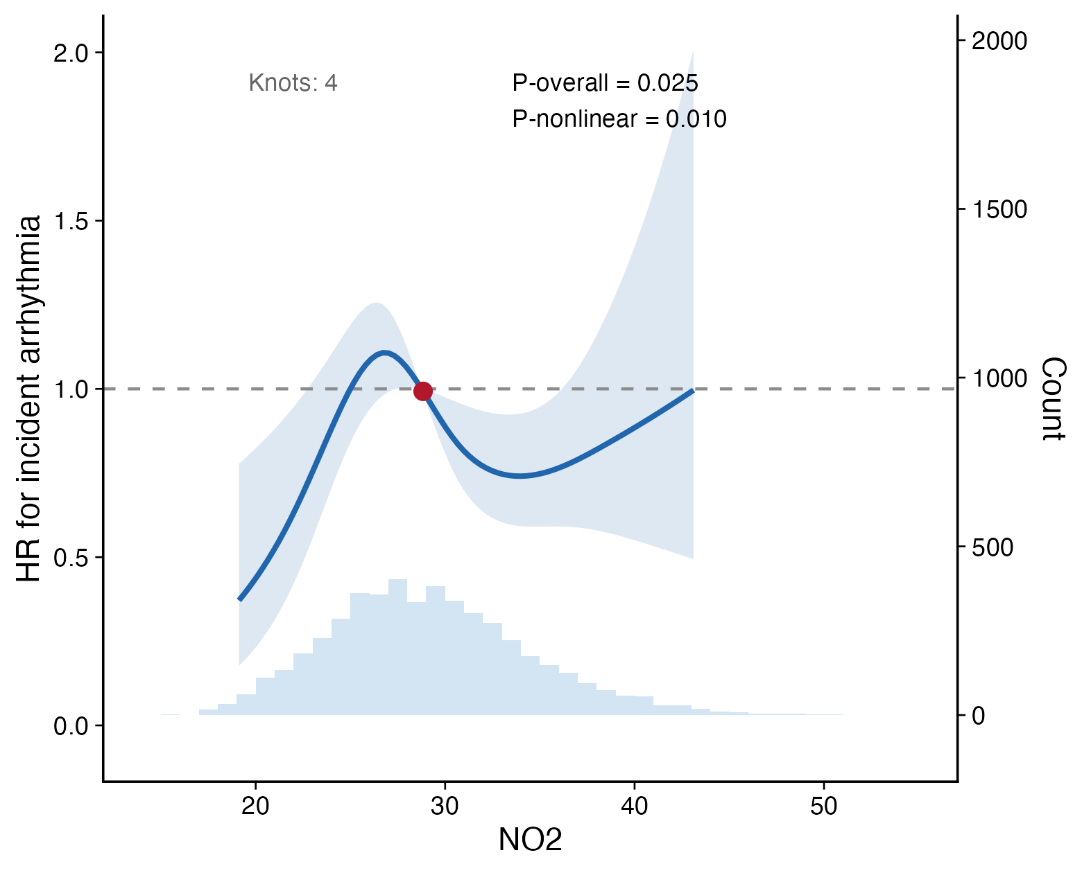
The solid curve is the estimated HR, and the shaded band is the 95% confidence interval. The dashed horizontal line indicates HR = 1. P-overall tests whether the exposure is associated with the outcome, while P-nonlinear tests whether the exposure-response shape deviates from linearity.

Logistic RCS for binary outcomes

For a binary endpoint, set model_type = "logistic" and provide outcome. The y-axis is an odds ratio relative to the reference exposure value.

rcs_pm25 <- run_rcs(
  data = analysis_data,
  exposure = "pm25",
  covariates = c("age", "sex", "tdi"),
  model_type = "logistic",
  outcome = "outcome_status",
  backend = "ns",
  knots = 4
)

plot_rcs(
  rcs_pm25,
  distribution = "density",
  xlab = "PM2.5",
  ylab = "OR for incident arrhythmia"
)

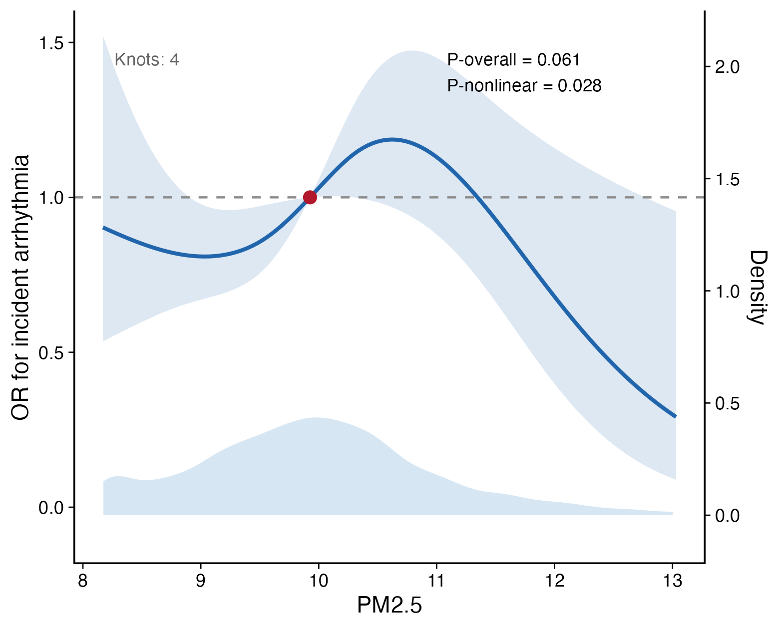
This model ignores follow-up time and treats the outcome as a binary status, so it is best suited to cross-sectional or fixed-window binary outcomes.

Linear RCS for continuous outcomes

For continuous outcomes, set model_type = "linear". The curve shows the difference in the outcome relative to the reference exposure value.

rcs_nox_bmi <- run_rcs(
  data = analysis_data,
  exposure = "nox",
  covariates = c("age", "sex", "tdi"),
  model_type = "linear",
  outcome = "bmi",
  backend = "ns",
  knots = 4
)

plot_rcs(
  rcs_nox_bmi,
  distribution = "rug",
  xlab = "NOx",
  ylab = "Difference in BMI"
)

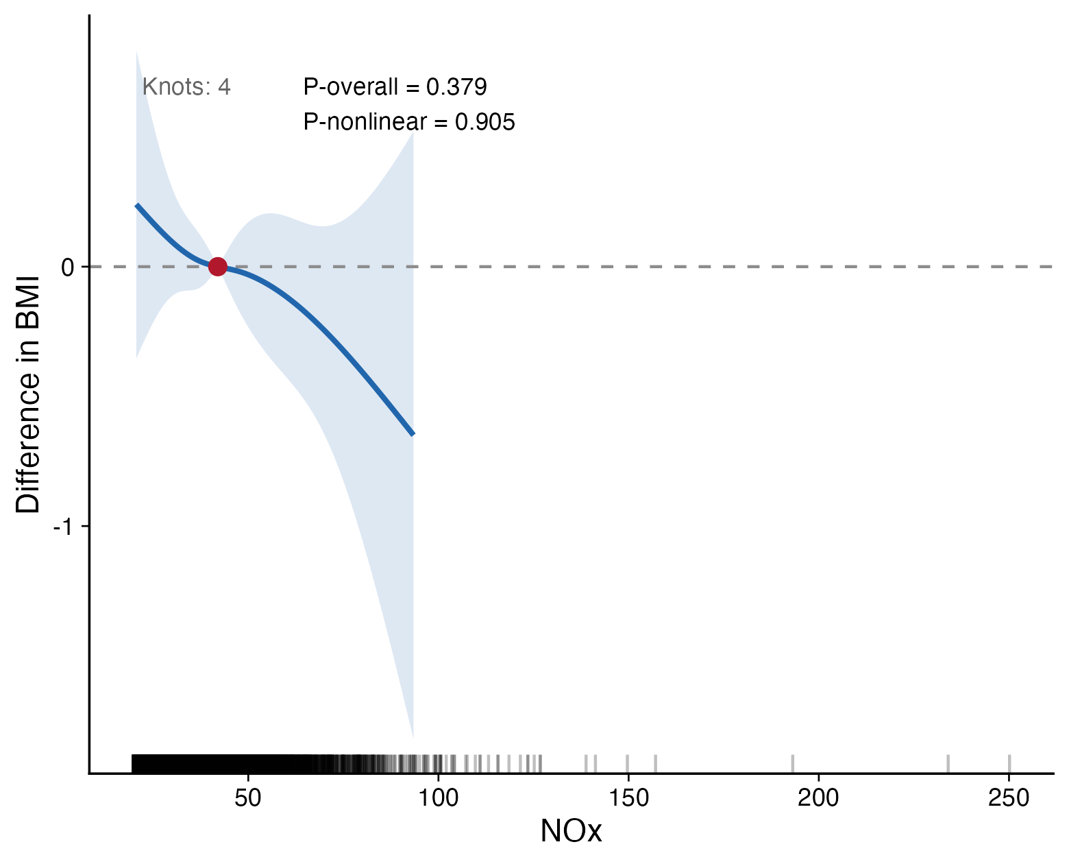
When the curve stays close to zero and the nonlinear P value is not significant, there is little evidence for a nonlinear exposure-response relationship.

Practical notes for RCS

• Prefer continuous exposures on their original scale unless a transformation is clinically meaningful.
• Avoid interpreting unstable tails when few participants are exposed at the extremes; trim_quantiles = c(0.01, 0.99) is used by default.
• Report the reference value, knot count, overall P value, nonlinear P value, adjustment covariates, and model family.
• Use backend = "rms" for formal manuscript analyses when the rms package is available; use backend = "ns" for lightweight examples and smoke tests.

Subgroup analysis

run_subgroup_analysis() estimates an interaction p-value from a full model containing an exposure-by-subgroup term, then refits separate models within each subgroup level and returns a harmonised table of effect estimates, confidence intervals, and interaction statistics.

Five model families are supported via the model_type argument:

model_type	Fitting function	Effect estimate
"cox"	survival::coxph()	Hazard ratio (HR)
"logistic"	stats::glm(binomial)	Odds ratio (OR)
"linear"	stats::lm()	Beta (mean difference)
"glm"	stats::glm(family)	Ratio (log/logit link) or beta (identity)
"negbin"	MASS::glm.nb()	Incidence rate ratio (IRR)

Time-to-event outcome

subgroup_res <- run_subgroup_analysis(
  data       = survival_data,
  exposure   = "smoking_status",
  subgroup_var = "sex",
  model_type = "cox",
  endpoint   = c("follow_up_time", "incident_status"),
  covariates = c("age", "bmi", "ethnic")
)

subgroup_res

Count outcome (Poisson GLM)

Use model_type = "glm" with family = "poisson" for count outcomes. The estimate column returns the incidence rate ratio (exp(beta)) when the family uses a log link.

subgroup_glm <- run_subgroup_analysis(
  data         = analysis_data,
  exposure     = "smoking_status",
  outcome      = "hospitalisation_count",
  subgroup_var = "sex",
  model_type   = "glm",
  family       = "poisson",
  covariates   = c("age", "bmi", "ethnic")
)

For overdispersed count outcomes, substitute model_type = "negbin" (no family argument required).

subgroup_nb <- run_subgroup_analysis(
  data         = analysis_data,
  exposure     = "smoking_status",
  outcome      = "hospitalisation_count",
  subgroup_var = "sex",
  model_type   = "negbin",
  covariates   = c("age", "bmi", "ethnic")
)
# estimate column = IRR = exp(beta); theta (dispersion) is reported per model

Multiple subgroup variables

For multiple subgroup variables, use run_multi_subgroup() and visualize the result with plot_forest().

subgroup_all <- run_multi_subgroup(
  data         = analysis_data,
  exposure     = "smoking_status",
  subgroup_vars = c("sex", "age_group", "bmi_group"),
  model_type   = "cox",
  endpoint     = c("follow_up_time", "incident_status"),
  covariates   = c("age", "bmi", "ethnic")
)

plot_forest(
  subgroup_all,
  estimate_col = "estimate",
  lower_col    = "lower95",
  upper_col    = "upper95",
  null_value   = 1,
  log_scale    = TRUE
)

The same model_type and family arguments apply to run_multi_subgroup().

Interaction p-value notes

• For single-level binary subgroups the interaction p-value comes from the Wald test on the single interaction coefficient.
• For multi-level factors a likelihood-ratio test (LRT) is used: the full model with all interaction terms is compared against the main-effects model via stats::anova(). Quasi-likelihood families fall back to an F-test.
• When the exposure has no variation within a subgroup level, the function returns NA for the effect estimate and issues a warning rather than stopping.

Propensity score analysis

Propensity score methods can be used when comparing an exposure or treatment group in observational data. The workflow is: estimate propensity scores, perform matching or weighting, then fit the outcome model.

ps_data <- estimate_propensity_score(
  data = analysis_data,
  treatment = "exposure_group",
  covariates = c("age", "sex", "bmi", "smoking_status", "ethnic"),
  method = "logistic"
)

matched_data <- match_propensity(
  data = ps_data,
  treatment = "exposure_group",
  ps_col = "ps",
  ratio = 1,
  caliper = 0.20
)

For IPTW analyses, use calculate_weights() followed by run_weighted_analysis().

weighted_data <- calculate_weights(
  data = ps_data,
  treatment = "exposure_group",
  ps_col = "ps",
  weight_type = "ATE",
  stabilized = TRUE
)

weighted_res <- run_weighted_analysis(
  data = weighted_data,
  exposure = "exposure_group",
  model_type = "cox",
  endpoint = c("follow_up_time", "incident_status"),
  weight_col = "weight"
)

weighted_res

Mediation analysis

run_mediation() wraps regression-based mediation analysis and supports linear, logistic, and Cox outcomes. It is useful when testing whether an exposure effect is partly explained through an intermediate variable.

med_res <- run_mediation(
  data = analysis_data,
  exposure = "smoking_status",
  mediator = "inflammatory_marker",
  outcome = "follow_up_time",
  outcome_type = "cox",
  endpoint = c("follow_up_time", "incident_status"),
  mediator_type = "continuous",
  covariates = c("age", "sex", "bmi", "ethnic"),
  exposure_levels = c(0, 1),
  boot = TRUE,
  boot_n = 1000
)

summary(med_res)

For screening several candidate mediators, use run_multi_mediator().

multi_med <- run_multi_mediator(
  data = analysis_data,
  exposure = "smoking_status",
  mediators = c("bmi", "crp", "hba1c"),
  outcome = "follow_up_time",
  outcome_type = "cox",
  endpoint = c("follow_up_time", "incident_status"),
  covariates = c("age", "sex", "ethnic")
)

multi_med

Practical notes

• Keep the adjustment set consistent with the main analysis unless the advanced analysis has a specific causal estimand.
• Check subgroup sample sizes and event counts before interpreting interaction p-values.
• Inspect propensity score overlap and covariate balance before reporting matching or weighting results.
• For mediation analysis, define the temporal and biological ordering of exposure, mediator, and outcome before model fitting.